Backing in to Confusion Matrix From False Positive Rate
Demystifying the Confusion Matrix Using a Business Example
A deep dive in confusion matrix, understanding the threshold,Area Under Curve(AUC) of ROC and their major impact on model evaluation.
![]()
You have just started machine learning and completed Supervised Linear Regression. Now you're able to build models with an okay-ish accuracy score. Now you move on to a classification model. You train the model and test it on the validation(test) data and voila, you're getting a whopping 91% accuracy score. But is accuracy the correct method of evaluation for your model? A Confusion Matrix will answer that question. There are many tutorials over the internet that will explain what confusion matrix is. This article will help you understand how businesses use confusion matrix analysis for their business solutions.
Wh a t is a Confusion Matrix?
A Confusion Matrix in simple terms contain the counts of our predicted data divided in 4 parts with respect to original data. It can be formed for a classification problem.
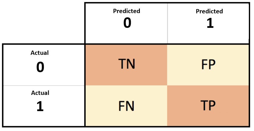
Lets understand the four parts using the example of spam filter. There are emails which are spam and not spam. Our spam filter will predict this.
1) True Negatives(TN): Originally non spam, predicted as non spam.
2) True Positives(TP): Originally spam, predicted as spam.
3) False Negative(FN): Originally a spam, predicted as non-spam.
4) False Positive(FP): Originally not a spam, predicted as a spam.
We can clearly see that TN and TP are correct predictions of our model and that accuracy can be calculated by: (TN+TP)/(total predictions). But companies rarely make decisions purely based on the accuracy score. There are many values derived from the confusion matrix such as sensitivity, specificity, recall, precision etc. that are preferred according to the business problem in hand. We can find the formulas for these performance metrics easily online. Let us now try to understand the importance of these point metrics using the business scenario of a bank trying to predict loan defaulters.
Bank Loan Defaulters' Confusion Matrix Evaluation
A bank creates a model to predict if a customer is a defaulter or not using its previous database. Here TN is actually and predicted as a non-defaulter, TP is actually and predicted as a defaulter. The errors of the model are FN and FP, where FN is actually a defaulter but predicted as a non-defaulter and FP is actually a non-defaulter predicted as defaulter.
In this case the company will keep an eye on two parameters:
1) True Positive Rate(TPR) : A true positive rate also known as sensitivity. In this case it will be, TP/(TP+FN). This metric will show us that out of all actual defaulters how many are predicted correctly. The bank will need a high value for this. Ideally it should be 1, because it will be beneficial for the bank if they can predict a defaulter and reject their application with 100 percent certainty.
2) False Positive Rate(FPR) : False positive rate is given by (FP/TN+FP), also known as as 1-specificity. This metric will show us that out of all non-defaulters how many are predicted as defaulters by the ML model. A low value for FPR is preferred. Ideally it should be zero because a high value will mean that the bank will reject potentially good customers if the ML model is implemented, thereby reducing the overall business of the bank.
Threshold Value and its Impact on Confusion Matrix
One thing that we can understand is that Confusion Matrix can be analysed according to the business problem in hand. Let us now try to understand how Confusion Matrix is formed. As we can see in the figure we have a set of Y-original and our model gives Y-probability as the output of the classification problem. Here Y-probability is the probability of Y being 1(defaulter) or 0(non-defaulter) according to our example.
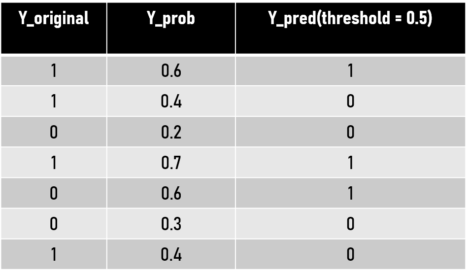
We can set a threshold value to classify all the values greater than threshold as 1 and lesser then that as 0. That's how the Y is predicted and we get 'Y-predicted'. The default value for threshold on which we generally get a Confusion Matrix is 0.50. This is where things start to get interesting. We can alter this threshold value. A change in the threshold value will see a change in predicted values of Y, hence the new confusion matrix will be different and more importantly TPR and FPR values will also change. Therefore we can visualise that for every unique value of a threshold we'll get different TPR and FPR value each. When these different TPR(sensitivity) and FPR(1-specificity) values are plotted on a scatter plot and a line is passed through them we get what we is famously called Receiver Operating Characteristic(ROC) curve.
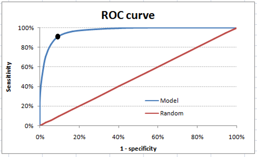
The ROC curve is different for different classification machine learning models. Just like sensitivity or accuracy, the area under curve(AUC) of ROC curve is treated as a very valuable metric to evaluate the model. The ROC in the figure has a high AUC. We can also see there's a point on the graph where TPR(sensitivity) is quite high and FPR(1-specificity) is dramatically low. If we go back and look at our business need, we needed a high TPR and low FPR that is exactly what we are getting from that point on this ROC. The threshold corresponding to that point can be said to be the best threshold value. But in real life scenarios, building a model with a very high AUC is not always possible. This is what a decent classification model's ROC will look like:
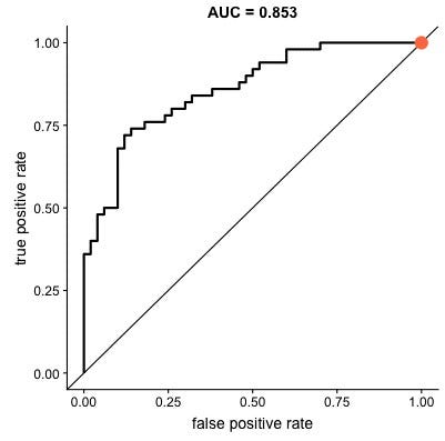
Looking at the graph, we can understand that to achieve a good True Positive Rate, False Positive Rate will also have to be raised. Therefore a trade-off has to be done between them. Now coming to the business part, the bank efficiently is balancing between reducing defaulters(increasing TPR) and reducing wrong classification of good customers as probable defaulters(lowering FPR). Therefore the organisation in this case can't just rely on the accuracy of the model. A deep analysis of the confusion matrix and connecting it with the business problem is required before jumping to any conclusions and making business decisions. Hence, after finalizing the TPR and FPR values the corresponding threshold value can easily be traced back and that will be used for the final prediction of the customer type(Y_pred). We can now understand how different business problems will require different analysis for proper model building.
Backing in to Confusion Matrix From False Positive Rate
Source: https://towardsdatascience.com/demystifying-confusion-matrix-29f3037b0cfa
0 Response to "Backing in to Confusion Matrix From False Positive Rate"
Post a Comment